library(tidyverse)

basic_plot <- ggplot(palmerpenguins::penguins %>%
                       filter(!is.na(flipper_length_mm)),
                     aes(x = island, y = flipper_length_mm)) +
  ggbeeswarm::geom_beeswarm(aes(fill = species,
                                size = body_mass_g),
                            shape = 21,
                            colour = "#FFFFFF",
                            alpha = 0.7) +
  colorblindr::scale_fill_OkabeIto() +
  guides(size = "none") +
  labs(title = "Only on Dream do penguins of different species share\nsimilar flipper lengths",
       subtitle = "Each column represents the penguin population of an island. Each dot is a penguin;
the larger the dot, the heavier the penguin. The Adelie penguins live on all three
islands. They share Biscoe with the longer-beflippered Gentoos, and Dream with
the equally-beflippered Chinstraps.",
       caption = "Data from {palmerpenguins}",
       x = "Island",
       y = "Flipper length",
fill = "")Variations on a ggtheme: Applying a unifying aesthetic to your plots
data-visualisation
dataviz-design-system
r-how-to
NHS-R Community Conference | Three reasons why you should apply a bespoke ggplot theme to your plots & how to do that
For those of us who need to know the answers before scrolling through a slide deck, here are the three reasons why I think you should consider using a bespoke ggplot theme for your plots!
- Add text hierarchy to help orient readers
- Give everything some space to breathe
- Effortlessly create aesthetic consistency throughout your data project
Recording
View the rest of the talks from Day 1 of the NHS-R 2022 Conference here.
Slides
Full code
The basic plot
Customising the theme()
First, some colours to improve text hierarchy:
dark_text <- "#1A242F"

monochromeR::generate_palette(
  dark_text,
  "go_lighter",
  n_colours = 5,
  view_palette = TRUE
)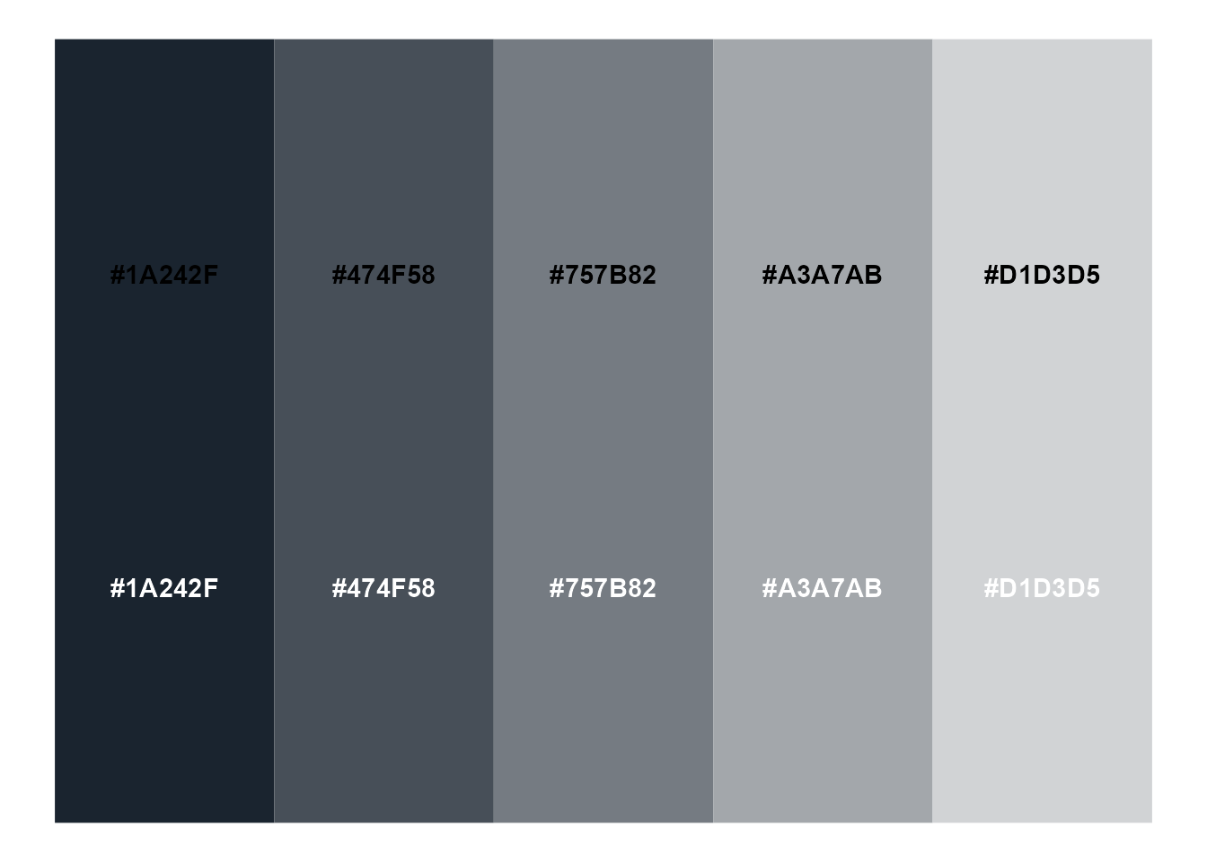
[1] "#1A242F" "#474F58" "#757B82" "#A3A7AB" "#D1D3D5"mid_text <- monochromeR::generate_palette(
dark_text, "go_lighter",
n_colours = 5)[2]
light_text <- monochromeR::generate_palette(
dark_text, "go_lighter",
n_colours = 5)[3]Then, let’s customise the theme:
basic_plot +
  theme_minimal(base_size = 12) +
  theme(text = element_text(colour = mid_text, family = "BrandonText", lineheight = 1.1),
        plot.title = element_text(colour = dark_text, family = "EnriquetaSB", size = rel(1.6), margin = margin(12, 0, 8, 0)),
        plot.subtitle = element_text(size = rel(1.1), margin = margin(4, 0, 0, 0)),
        axis.text.y = element_text(colour = light_text, size = rel(0.8)),
        axis.title.y = element_text(size = 12, margin = margin(0, 4, 0, 0)),
        axis.text.x = element_text(colour = mid_text, size = 12),
        axis.title.x = element_blank(),
        legend.position = "top",
        legend.justification = 1,
        panel.grid = element_line(colour = "#F3F4F5"),
        plot.caption = element_text(size = rel(0.8), margin = margin(8, 0, 0, 0)),
        plot.margin = margin(0.25, 0.25, 0.25, 0.25,"cm"))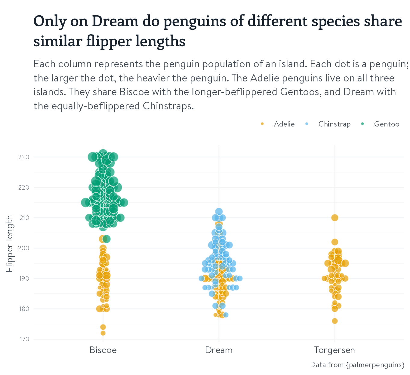
Packaging the theme up as a reusable function
theme_nhsr_demo <- function(base_size = 12,
                            dark_text = "#1A242F") {

  mid_text <-  monochromeR::generate_palette(dark_text, "go_lighter", n_colours = 5)[2]
  light_text <-  monochromeR::generate_palette(dark_text, "go_lighter", n_colours = 5)[3]

  theme_minimal(base_size = base_size) +
    theme(text = element_text(colour = mid_text, family = "BrandonText", lineheight = 1.1),
          plot.title = element_text(colour = dark_text, family = "EnriquetaSB", size = rel(1.6), margin = margin(12, 0, 8, 0)),
          plot.subtitle = element_text(size = rel(1.1), margin = margin(4, 0, 0, 0)),
          axis.text.y = element_text(colour = light_text, size = rel(0.8)),
          axis.title.y = element_text(size = 12, margin = margin(0, 4, 0, 0)),
          axis.text.x = element_text(colour = mid_text, size = 12),
          axis.title.x = element_blank(),
          legend.position = "top",
          legend.justification = 1,
          panel.grid = element_line(colour = "#F3F4F5"),
          plot.caption = element_text(size = rel(0.8), margin = margin(8, 0, 0, 0)),
          plot.margin = margin(0.25, 0.25, 0.25, 0.25,"cm"))
}
Applying it to various plots
mtcars
mtcars %>%
  ggplot(aes(x = cyl, y = disp,
             colour = as.character(am))) +
  geom_point(aes(size = mpg),
             shape = 15,
             alpha = 0.8) +
  scale_x_continuous(breaks = c(4, 6, 8)) +
  labs(title = "I don't know enough about cars...",
       subtitle = "But I know lots of people use this dataset!",
       caption = "Data from mtcars",
       colour = "am") +
  theme_nhsr_demo()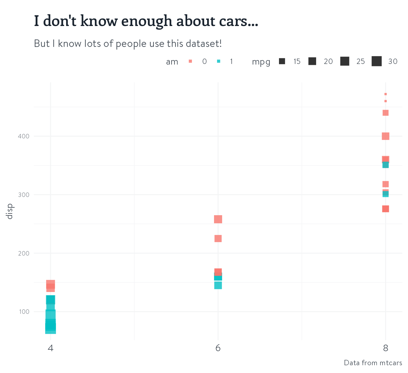
Orange
Orange %>%
  mutate(label_hjust = rep(c(0.9, 0.7, 0.9, 0.8, 0.7), 7)) %>%
  ggplot(aes(x = age, y = circumference,
             colour = Tree)) +
  geomtextpath::geom_textline(aes(label = paste0("Tree #", Tree),
                                  hjust = label_hjust),
                              show.legend = FALSE,
                              size = 5,
                              family = "Enriqueta") +
  labs(title = "Five little orange trees growing at their own pace",
       subtitle = "As the time keeps ticking on, they're taking up more space\nWatching their great journey, one question comes to mind\nDo you think Tree number 4 will leave the others behind?",
       caption = "Data from Orange",
       y = "Circumference",
       x = "Age (in days)") +
  theme_nhsr_demo() +
  theme(axis.text.x = element_text(colour = light_text,
                                   size = rel(0.8)),
        axis.title.x = element_text(margin = margin(8, 0, 0, 0)))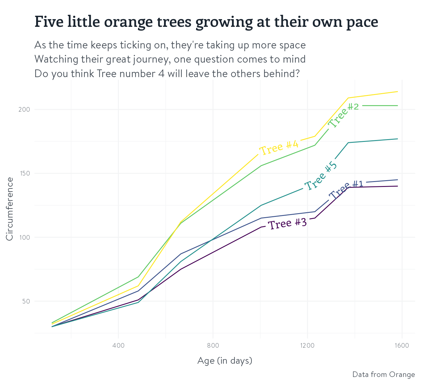
ToothGrowth
ToothGrowth %>%
  mutate(supplement = factor(case_when(supp == "VC" ~ "Vitamin C",
                                       supp == "OJ" ~ "Orange Juice"))) %>%
  ggplot() +
  geom_boxplot(aes(group = dose,
                   y = len,
                   alpha = dose,
                   fill = supplement),
               show.legend = FALSE,
               colour = light_text) +
  facet_wrap( ~ supplement) +
  scale_fill_manual(values = list(`Orange Juice` = "#e3ad0a",
                                  `Vitamin C` = "#fd6a0d")) +
  labs(title = "The growth of the odontoblast of the incisor teeth as a\ncriterion of vitamin C intake of the guinea pig",
       subtitle = "Is that a win for Orange Juice? Looks like it to me!
       ",
       x = "Dose",
       y = "",
       caption = "Data from ToothGrowth") +
  theme_nhsr_demo() +
  theme(axis.text.x = element_text(colour = light_text, size = rel(0.8)),
    axis.title.x = element_text(margin = margin(8, 0, 0, 0)),
    strip.background = element_rect(fill = "#F3F4F5", color = "#FFFFFF"),
    strip.text = element_text(family = "Enriqueta",size = 14))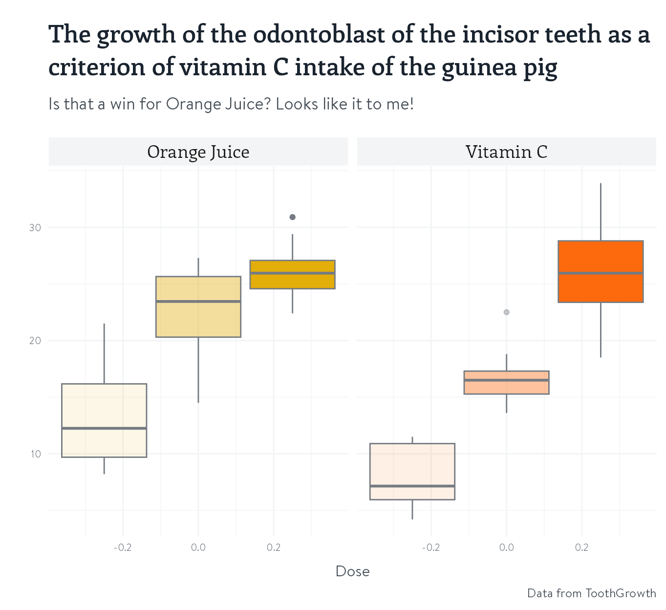
Reuse
Citation
For attribution, please cite this work as:
Thompson, Cara. 2022. “Variations on a Ggtheme: Applying a
Unifying Aesthetic to Your Plots.” November 16, 2022. https://www.cararthompson.com/talks/nhsr2022-ggplot-themes/.